How Python and Go Manage Dynamic Array Growth
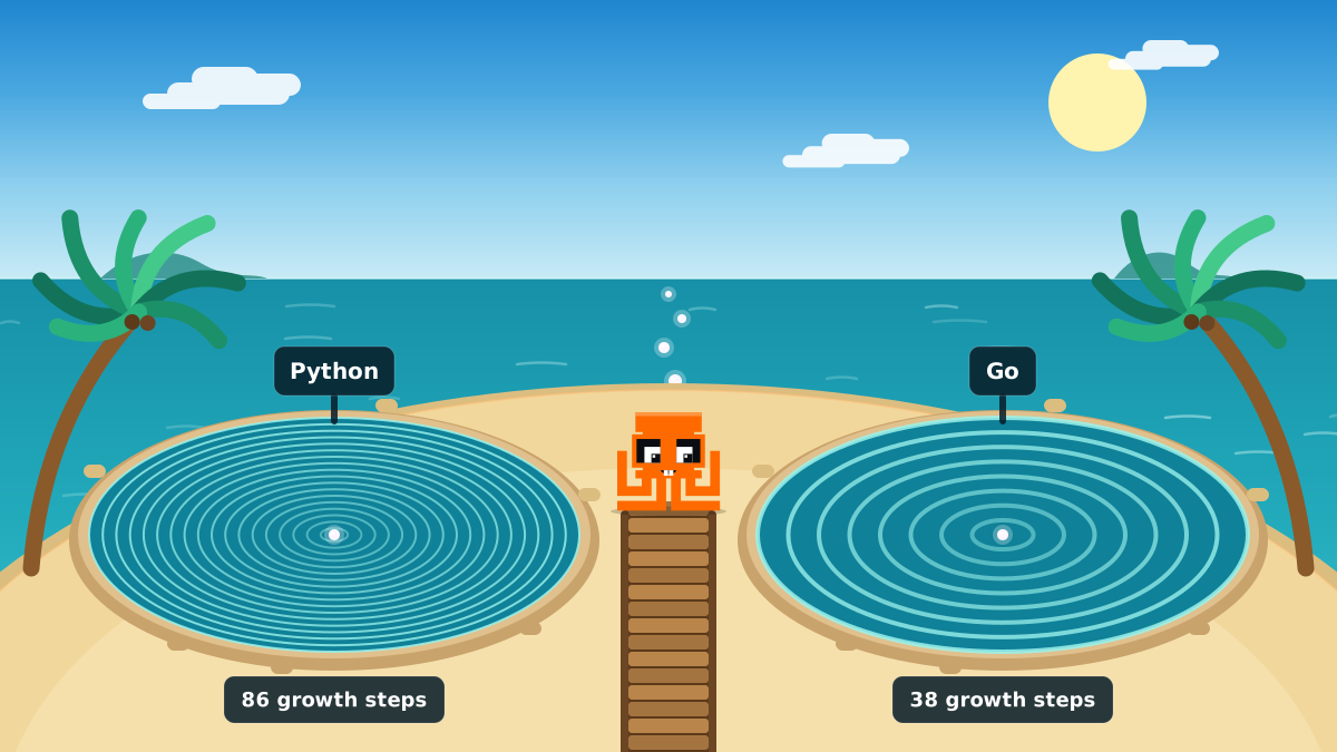
We appended one million elements to Python lists and Go slices. Python increased capacity 86 times; Go did it 38 times. Their final capacities were only 340 slots apart.

I wrote two small programs with the same job: start with an empty collection, append one million elements one at a time, and record every change in capacity.
The first results were different enough to catch my attention:
- Python 3.13.5: 86 capacity increases
- Go 1.23.2: 38 capacity increases
Go needed fewer than half as many growth steps. I expected its final slice to have substantially more spare room than Python's list.
Then I looked at the final capacities.
| Runtime | Capacity after 1,000,000 appends | Unused slots |
|---|---|---|
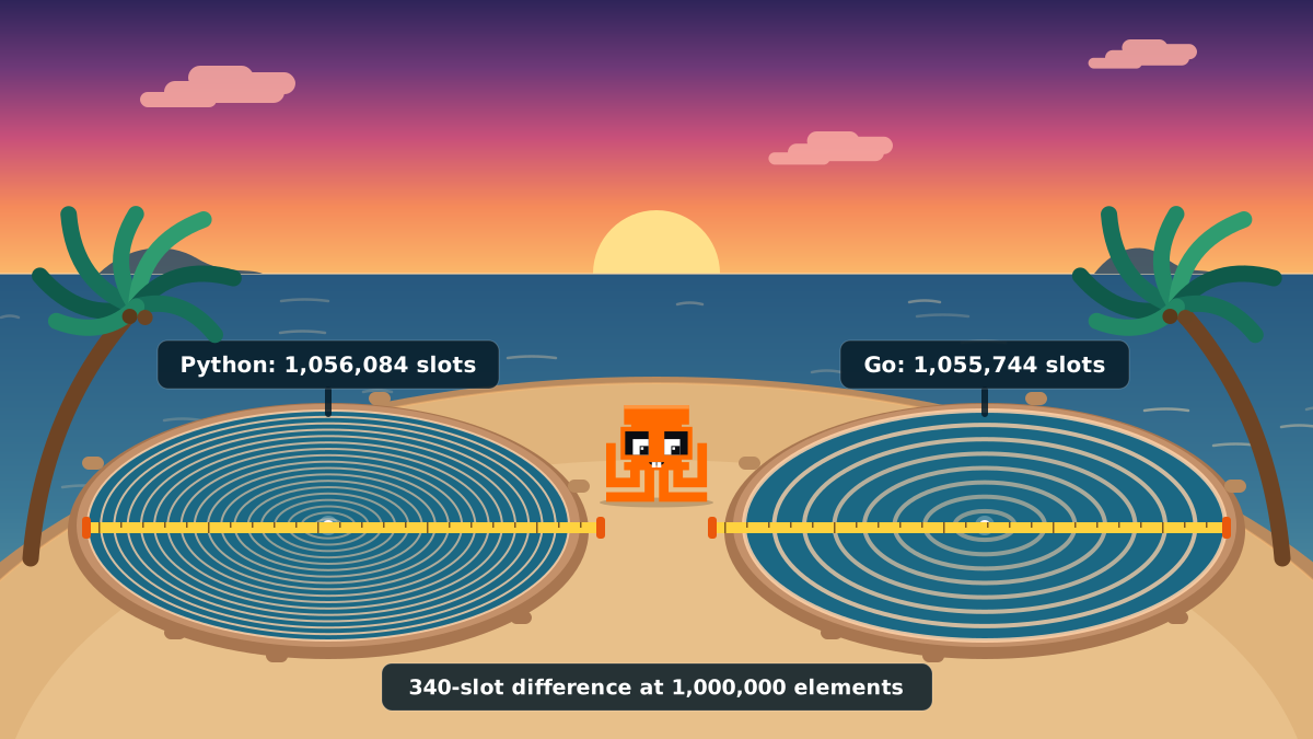
| Python 3.13.5 | 1,056,084 | 56,084 |
| Go 1.23.2 | 1,055,744 | 55,744 |
They ended up 340 slots apart, despite taking very different paths to get there.
This made me curious about the allocation rules inside each runtime, and what those rules tell us about the cost of appending to a dynamic array.
Measuring growth
The Python test appends one million values and uses sys.getsizeof() to observe when the list's allocated pointer array grows:
import sys

base_size = sys.getsizeof([])
items = []
old_capacity = 0
changes = []

for length in range(1, 1_000_001):
    items.append(length)
    capacity = (sys.getsizeof(items) - base_size) // 8
    if capacity != old_capacity:
        changes.append((length, capacity))
        old_capacity = capacity

print(len(changes), changes[-1])
# 86 (938737, 1056084)
The calculation relies on the measured 64-bit CPython build, where each list slot holds an eight-byte object reference. It measures list slot capacity, not the memory consumed by the integers stored in the list.
Go exposes slice capacity directly through cap():
package main

import "fmt"

func main() {
    items := make([]int, 0)
    oldCap := cap(items)
    changes := make([][2]int, 0)

    for length := 1; length <= 1_000_000; length++ {
        items = append(items, length)
        if cap(items) != oldCap {
            changes = append(changes, [2]int{length, cap(items)})
            oldCap = cap(items)
        }
    }

    fmt.Println(len(changes), changes[len(changes)-1])
    // 38 [843777 1055744]
}
I ran both programs on Linux x86-64. The measurements compare capacity-growth strategies, rather than total memory consumption or execution speed: a Go []int stores integers directly, while a Python list stores references to Python objects.
The first few steps
Python's initial growth pattern looks like this:
Append #   New capacity
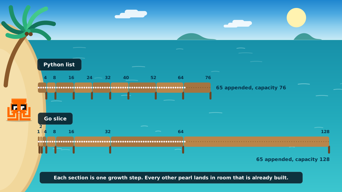
1          4
5          8
9          16
17         24
25         32
33         40
41         52
53         64
65         76
77         92
Go starts differently:
Append #   New capacity
1          1
2          2
3          4
5          8
9          16
17         32
33         64
65         128
129        256
257        512
The patterns explain much of the difference in growth-event counts.
Go doubles capacity repeatedly at small sizes. Python grows rapidly at first, then switches to much smaller proportional increments.
Both are reserving room for future appends. If they allocated exactly one new slot every time the list or slice became full, appending a million elements would require an enormous amount of repeated allocation and copying.
The spare capacity is what makes most appends cheap.
Why Python grows in smaller steps
The relevant CPython implementation is in Objects/listobject.c.
The allocation calculation is compact:
new_allocated = ((size_t)newsize + (newsize >> 3) + 6) & ~(size_t)3;In ordinary terms, the expression adds roughly 12.5% to the requested size, includes a small fixed amount of padding, and rounds the result to a multiple of four slots. The implementation also has special handling for larger one-shot changes in list length.
The source comments describe this as mild over-allocation, intended to provide good amortized append behavior without reserving too much unnecessary memory.
As the list becomes large, its growth steps remain comparatively conservative. Here are the final ten growth events from the experiment:
325,189 ->   365,840
365,841 ->   411,576
411,577 ->   463,028
463,029 ->   520,912
520,913 ->   586,032
586,033 ->   659,292
659,293 ->   741,708
741,709 ->   834,428
834,429 ->   938,736
938,737 -> 1,056,084
Python buys a relatively modest amount of headroom at each step. That means more growth events, but usually less unused capacity immediately after an expansion than a more aggressive strategy would create.
Why Go grows differently
Go's implementation lives in runtime/slice.go.
Its nextslicecap function starts by doubling smaller slices and gradually transitions toward approximately 1.25x growth for large ones:
const threshold = 256
if oldCap < threshold {
    return doublecap
}

for {
    newcap += (newcap + 3*threshold) >> 2
    if uint(newcap) >= uint(newLen) {
        break
    }
}
The threshold is part of a smooth transition, rather than an abrupt switch to multiplying every capacity by exactly 1.25.
There's another detail in Go's runtime: after calculating a target, the allocator can round the requested allocation to one of its size classes. That can change the resulting capacity.
You can see the combined effect in the experiment:
Append #   New capacity
513        848
849        1280
1281       1792
1793       2560
2561       3408
3409       5120
5121       7168
7169       9216
9217       12288
12289      16384
These aren't simple powers of two anymore. Go's growth calculation and allocation rounding both influence the result.
The strategy leaves plenty of headroom early on, while reducing the relative growth rate as slices become larger. Across our million appends, Go crossed just 38 distinct capacity thresholds.
Two paths to almost the same result
The final capacities deserve a second look:
- Python: 1,056,084
- Go: 1,055,744
The tiny difference at one million elements is a consequence of where that particular length happened to fall within each runtime's sequence of capacity thresholds. It isn't a promise that the capacities will remain close at other lengths.
In fact, their final growth events occurred at different points. Python last grew when append 938,737 exceeded its previous capacity. Go last grew at append 843,777.
After that, each collection had enough space to accept the remaining appends without another capacity increase.
That is how two very different histories produced nearly identical final numbers.
What this tells us about append
Dynamic arrays are a standard example of amortized constant-time operations.
Most appends simply write an element into an existing allocation. Occasionally, an append exceeds capacity, and the runtime must arrange for a larger backing array and preserve the existing elements.
In our runs:
| Runtime | Appends | Capacity increases | Appends without a capacity increase |
|---|---|---|---|
| Python | 1,000,000 | 86 | 999,914 |
| Go | 1,000,000 | 38 | 999,962 |
The rare growth events can be expensive, but geometric growth spreads their costs over a much larger number of ordinary appends. That's the practical intuition behind the amortized analysis.
The table counts capacity changes, not physical memory moves. In particular, a memory allocator may sometimes extend an allocation in place. Still, the capacity changes are a useful way to see how often the runtime has to accommodate growth.
What changes when we know the final size?
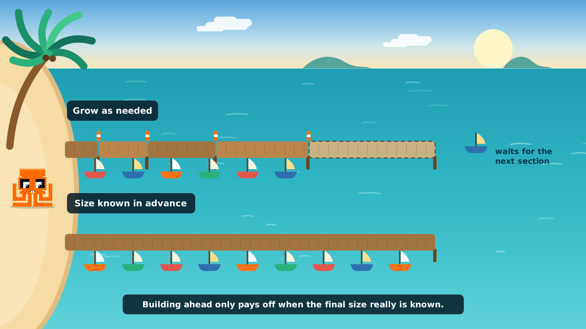
When the final size is predictable, we can avoid most or all of those intermediate growth events.
In Go, preallocating spare capacity is explicit:
items := make([]int, 0, 1_000_000)
for i := 0; i < 1_000_000; i++ {
    items = append(items, i)
}
The slice starts with length zero and capacity one million. Every append in this loop fits within the original allocation.
Python has a different interface. It doesn't offer a public list.reserve() method, but when we're going to fill a known number of positions, we can allocate the complete list and assign into it:
items = [None] * 1_000_000
for i in range(1_000_000):
    items[i] = i
Here, the list starts with length one million, rather than length zero with reserved capacity. The operation changes from append to indexed assignment, but it similarly avoids the staircase of list-capacity growth.
Neither approach is automatically the best choice for every program. Allocating a million positions up front makes sense when the workload is known; it wastes resources when the final collection might remain small. It is also worth measuring before making performance-sensitive changes.
A small experiment, a useful reminder
I expected Python and Go to differ. Python lists and Go slices have different public interfaces, different element representations, and different runtime implementations.
What surprised me was how close their capacities ended up after a million appends.
Looking at the source code made the result much easier to understand. Python chooses relatively small proportional growth steps. Go doubles early, transitions toward smaller proportional increases, and incorporates allocator rounding. Both strategies keep the common append path cheap by reserving space for future elements.
The final capacities happen to converge at one million elements, but the more interesting result is the different path each runtime took to get there.
It's easy to treat append as a single, constant-cost operation when writing application code. Most of the time, that's exactly how it feels. Underneath, though, the runtime is continually making small decisions about allocation, copying, and the value of spare room.
For me, watching those decisions play out was a more memorable explanation of amortized growth than any abstract formula.
Methodology and source code
- Environment: Linux x86-64, Python 3.13.5, Go 1.23.2.
- Workload: One million sequential appends to an initially empty CPython list and a Go
[]intslice. - Measurement: Python list slot capacity inferred from
sys.getsizeof()on the measured 64-bit build; Go capacity read withcap(). - Interpretation: Growth events and capacities, without making claims about relative speed or total process memory use.
Primary implementation references: